MSIBI: Simple Tutorial
Purpose
This tutorial will illustrate the process of stringing together multiple instances of msibi optimization runs. It is common for IBI and MSIBI methods to optimize forces in order of their relative strength, which typically means bond stretching is optimized first, followed by bond angles, then non-bonded pairs and dihedrals, where the potential learned from the previous step is included in the next optimization. The API for msibi is designed to make it straight-forward to follow this process. This tutorial is split into three sections:
Using a target trajectory of a single-chain simulation, an
msibi.Bondforce is optimized without including any additional forces.Using the same target trajectory, an
msibi.Angleforce is optimized. This optimization includes setting a harmonic bond-stretching force where the parameters were obtained from step 1.Using a target trajectory of a “bulk system” of oligomers, an
msibi.Pairforce is optimized. This includes setting a table potential for angle interactions (obtained from step 2) and a harmonic potential for bond-stretching (obtained from step 1).
Before running this tutorial, see the installation section of the documentation to ensure you have the software environment needed to run this notebook.
A note about MSIBI’s parameters:
There are several hyper-parameters available in MSIBI that can significantly affect the outcome of the final potentials. These include things such as sampling sizing and frequency (msibi.State.n_frames, msibi.State.sampling_stride, number of simulations steps per iteration), the alpha value used in weighting state points and damping potential corrections (msibi.State.alpha0), as well as smoothing choices such as how often to smooth the learned potential (e.g., between each MSIBI
iteration, or only once at the end), smoothing window and order (msibi.Force.smoothing_window and msibi.Force.smoothing_order). Therefore, when using MSIBI on your own systems, it is important to explore these parameters and understand the impact it can have on the final outcome.
Because of differences in software environments, it might be the case that your outputs differ from those shown in these examples. Try changing some of these parameters to see how it affects the final potentials and distribution matching.
A note about head and tail corrections:
The MSIBI method is only valid in regions of the sampled distribution that are non-zero. In order to extrapolate the learned potential across the entire range, correction functions are used for the head and tail regions. It is possible, either due to poor sampling, or to other parameter choices, that this fitting and correction procedure may fail. In these cases, try adjusting the parameters listed above and ensure the target trajectory is sufficiently sampled.
Target Trajectories
These examples use target simulations of simple Lennard-Jones (LJ) bead-spring models. In other words, these are already coarse-grained simulations, and the examples below “learn” the potential that was used in these target simulations. This is different from most applications of MSIBI, where the target trajectories are atomistic simulations that have had a coarse-grained mapping applied. In these cases, the coarse-grain potential is not known ahead of time, and the correctness of the learned potnetial is determined not just by structure-matching performance–which MSIBI optimizes against–but also other properties and behavior depending on the underlying systems and applications. To summarize, these examples suffice to illustrate the user interface and general process of using MSIBI to learn a coarse-grained forcefield, and using these simple systems allow this tutorial to do this without having to deal with complications from coarse-graining atomistic systems.
The target simulations used the following model:
Lennard Jones spheres are connected by harmonic bonds with the following interactions:
\(V_{bond}(l) = 0.5k_{l}(l - l_0)^2\)
\(V_{angle}(\theta) = 0.5k_{\theta}(\theta - \theta_0)^2\)
\(V_{nb}(r) = 4\epsilon\left[\left(\dfrac{\sigma}{r}\right)^{12} - \left(\dfrac{\sigma}{r}\right)^6\right]\)
with:
Parameter |
Value |
Description |
|---|---|---|
\(k_l\) |
500 |
Bond-stretching force constant |
\(l_0\) |
1.1 |
Equilibrium bond length |
\(k_{\theta}\) |
250 |
Bond-bending force constant |
\(\theta_0\) |
2.0 |
Equilibrium bond angle |
\(\epsilon\) |
1.0 |
Depth of non-bonded potential energy well |
\(\sigma\) |
1.0 |
Particle radius |
Bonds and angles are learned from a single chain of 20 beads in a low density box (i.e., vacuum) while pairs are learned from a “bulk” system of 50 oligomers with 6 beads each.
[1]:
import importlib.resources
import os

from msibi import State, Bond, Angle, Pair, MSIBI
import hoomd
import matplotlib.pyplot as plt
import numpy as np

import warnings

warnings.filterwarnings("ignore")

# NOTE: The 4 lines of code below are only necessary for this tutorial.
# They are needed to give a path to sample .gsd files used in this tutorial.
with importlib.resources.path(
    "msibi.tests.validation", "target_data", "chains"
) as target_dir:
    target_data_dir = target_dir
1) Optimizing a bond-stretching potential:
We will use a target trajectory consisting of a single chain simulation with a Lennard-Jones bead-spring model.
Preparing all of the classes needed to run MSIBI:
In this cell we make the following:
msibi.MSIBI: Object which acts as the context manager for the rest of the workflow.Here, we set the simulation methods (NVT), thermostat (MTTK) and neighborlist (Cell) to use.
We provide additional parameters of time step (dt), thermostat coupling constant (tau), and trajectory write out frequency (gsd_period).
These set the methods used during coarse-grained query simulations, and the write out frequency effects sampling results of distributions.
msibi.State: Object which stores the target trajectory, state point information (temperature), and sampling information (n_frames, sampling stride)Here we set information about the target trajectory such as the path to the target .gsd file, the temperature (kT) of the target trajectory, and state point name.
Parameters that are used for sampling the distributions are set here such as number of frames (n_frames), and step size between sampled frames (sampling_stride).
Finally, the state-point weighting factor (alpha), or in the case of a single-state point the damping factor, is set.
msibi.ForceObject which provides forces used in the coarse-grained query simulations.Here, we only include one bond-stretching force (
msibi.Bond), which is also the force being optimized (optimize=True).It is required to set an initial potential to use during MSIBI iterations. Here, we use the
set_polynomialmethod where we create a harmonic bond-stretching potential with initial parameters of \(x_0 = 1.3\sigma\), \(k2 = 200 \epsilon\), \(k3=0\), and \(k4=0\). By setting \(k3\) and \(k4\) to zero, this results in an initial “guess” potential of \(V(x) = 200(x-1.3)^2\)
[2]:
# Remove the states directory created by the previous run
!rm -r states/

optimizer = MSIBI(
    nlist=hoomd.md.nlist.Cell,
    integrator_method=hoomd.md.methods.ConstantVolume,
    thermostat=hoomd.md.methods.thermostats.MTTK,
    thermostat_kwargs={"tau": 0.1},
    method_kwargs={},
    dt=0.0001,
    gsd_period=500,
    seed=50,
)

state = State(
    name="single-chain",
    kT=4.0,
    traj_file=os.path.join(str(target_data_dir), "single-chain.gsd"),
    n_frames=100,
    sampling_stride=2,
    alpha0=0.4,
)

bond = Bond(
    type1="A",
    type2="A",
    optimize=True,
    nbins=60,
    smoothing_window=5,
    correction_fit_window=7,
    smoothing_order=1,
)
bond.set_polynomial(x_min=0.0, x_max=2.5, x0=1.3, k2=200, k3=0, k4=0)

optimizer.add_state(state)
optimizer.add_force(bond)
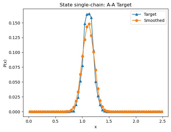
Let’s look at the target bond-length distribution, which is automatically calculated with the given
[3]:
bond.plot_target_distribution(state=state)
[4]:
optimizer.run_optimization(n_iterations=15, n_steps=5e5, backup_trajectories=False)
bond.smooth_potential()
---Optimization: 1 of 15---
Starting simulation 0 for state <class 'msibi.state.State'>; Name: single-chain; kT: 4.0; Alpha0: 0.4
Running on device <hoomd.device.CPU object at 0x15abd42f0>
Finished simulation 0 for state <class 'msibi.state.State'>; Name: single-chain; kT: 4.0; Alpha0: 0.4. TPS = 1404450.9860650373

Force: A-A, State: single-chain, Iteration: 0, Fit score:0.399579

---Optimization: 2 of 15---
Starting simulation 1 for state <class 'msibi.state.State'>; Name: single-chain; kT: 4.0; Alpha0: 0.4
Running on device <hoomd.device.CPU object at 0x15abd42f0>
Finished simulation 1 for state <class 'msibi.state.State'>; Name: single-chain; kT: 4.0; Alpha0: 0.4. TPS = 1453044.8554946892

Force: A-A, State: single-chain, Iteration: 1, Fit score:0.532632

---Optimization: 3 of 15---
Starting simulation 2 for state <class 'msibi.state.State'>; Name: single-chain; kT: 4.0; Alpha0: 0.4
Running on device <hoomd.device.CPU object at 0x15abd42f0>
Finished simulation 2 for state <class 'msibi.state.State'>; Name: single-chain; kT: 4.0; Alpha0: 0.4. TPS = 1411070.1273631896

Force: A-A, State: single-chain, Iteration: 2, Fit score:0.653474

---Optimization: 4 of 15---
Starting simulation 3 for state <class 'msibi.state.State'>; Name: single-chain; kT: 4.0; Alpha0: 0.4
Running on device <hoomd.device.CPU object at 0x15abd42f0>
Finished simulation 3 for state <class 'msibi.state.State'>; Name: single-chain; kT: 4.0; Alpha0: 0.4. TPS = 1452871.746293724

Force: A-A, State: single-chain, Iteration: 3, Fit score:0.751368

---Optimization: 5 of 15---
Starting simulation 4 for state <class 'msibi.state.State'>; Name: single-chain; kT: 4.0; Alpha0: 0.4
Running on device <hoomd.device.CPU object at 0x15abd42f0>
Finished simulation 4 for state <class 'msibi.state.State'>; Name: single-chain; kT: 4.0; Alpha0: 0.4. TPS = 1451062.90357687

Force: A-A, State: single-chain, Iteration: 4, Fit score:0.794526

---Optimization: 6 of 15---
Starting simulation 5 for state <class 'msibi.state.State'>; Name: single-chain; kT: 4.0; Alpha0: 0.4
Running on device <hoomd.device.CPU object at 0x15abd42f0>
Finished simulation 5 for state <class 'msibi.state.State'>; Name: single-chain; kT: 4.0; Alpha0: 0.4. TPS = 1442214.7803939553

Force: A-A, State: single-chain, Iteration: 5, Fit score:0.859579

---Optimization: 7 of 15---
Starting simulation 6 for state <class 'msibi.state.State'>; Name: single-chain; kT: 4.0; Alpha0: 0.4
Running on device <hoomd.device.CPU object at 0x15abd42f0>
Finished simulation 6 for state <class 'msibi.state.State'>; Name: single-chain; kT: 4.0; Alpha0: 0.4. TPS = 1442759.942058761

Force: A-A, State: single-chain, Iteration: 6, Fit score:0.897895

---Optimization: 8 of 15---
Starting simulation 7 for state <class 'msibi.state.State'>; Name: single-chain; kT: 4.0; Alpha0: 0.4
Running on device <hoomd.device.CPU object at 0x15abd42f0>
Finished simulation 7 for state <class 'msibi.state.State'>; Name: single-chain; kT: 4.0; Alpha0: 0.4. TPS = 1436876.5751759456

Force: A-A, State: single-chain, Iteration: 7, Fit score:0.914105

---Optimization: 9 of 15---
Starting simulation 8 for state <class 'msibi.state.State'>; Name: single-chain; kT: 4.0; Alpha0: 0.4
Running on device <hoomd.device.CPU object at 0x15abd42f0>
Finished simulation 8 for state <class 'msibi.state.State'>; Name: single-chain; kT: 4.0; Alpha0: 0.4. TPS = 1461761.7737602068

Force: A-A, State: single-chain, Iteration: 8, Fit score:0.950526

---Optimization: 10 of 15---
Starting simulation 9 for state <class 'msibi.state.State'>; Name: single-chain; kT: 4.0; Alpha0: 0.4
Running on device <hoomd.device.CPU object at 0x15abd42f0>
Finished simulation 9 for state <class 'msibi.state.State'>; Name: single-chain; kT: 4.0; Alpha0: 0.4. TPS = 1450679.7885489142

Force: A-A, State: single-chain, Iteration: 9, Fit score:0.944421

---Optimization: 11 of 15---
Starting simulation 10 for state <class 'msibi.state.State'>; Name: single-chain; kT: 4.0; Alpha0: 0.4
Running on device <hoomd.device.CPU object at 0x15abd42f0>
Finished simulation 10 for state <class 'msibi.state.State'>; Name: single-chain; kT: 4.0; Alpha0: 0.4. TPS = 1450540.90670411

Force: A-A, State: single-chain, Iteration: 10, Fit score:0.950947

---Optimization: 12 of 15---
Starting simulation 11 for state <class 'msibi.state.State'>; Name: single-chain; kT: 4.0; Alpha0: 0.4
Running on device <hoomd.device.CPU object at 0x15abd42f0>
Finished simulation 11 for state <class 'msibi.state.State'>; Name: single-chain; kT: 4.0; Alpha0: 0.4. TPS = 1453171.5469011115

Force: A-A, State: single-chain, Iteration: 11, Fit score:0.954526

---Optimization: 13 of 15---
Starting simulation 12 for state <class 'msibi.state.State'>; Name: single-chain; kT: 4.0; Alpha0: 0.4
Running on device <hoomd.device.CPU object at 0x15abd42f0>
Finished simulation 12 for state <class 'msibi.state.State'>; Name: single-chain; kT: 4.0; Alpha0: 0.4. TPS = 1443234.6930528455

Force: A-A, State: single-chain, Iteration: 12, Fit score:0.977684

---Optimization: 14 of 15---
Starting simulation 13 for state <class 'msibi.state.State'>; Name: single-chain; kT: 4.0; Alpha0: 0.4
Running on device <hoomd.device.CPU object at 0x15abd42f0>
Finished simulation 13 for state <class 'msibi.state.State'>; Name: single-chain; kT: 4.0; Alpha0: 0.4. TPS = 1445491.9442733945

Force: A-A, State: single-chain, Iteration: 13, Fit score:0.965263

---Optimization: 15 of 15---
Starting simulation 14 for state <class 'msibi.state.State'>; Name: single-chain; kT: 4.0; Alpha0: 0.4
Running on device <hoomd.device.CPU object at 0x15abd42f0>
Finished simulation 14 for state <class 'msibi.state.State'>; Name: single-chain; kT: 4.0; Alpha0: 0.4. TPS = 1446654.6112115732

Force: A-A, State: single-chain, Iteration: 14, Fit score:0.973053
Examining the results
Here we will view the evolution of the potential obtained from MSIBI (
bond.plot_potential_history)Compare against the known potential used
Compare the target bond-length distribution against the distribution obtained from MSIBI.
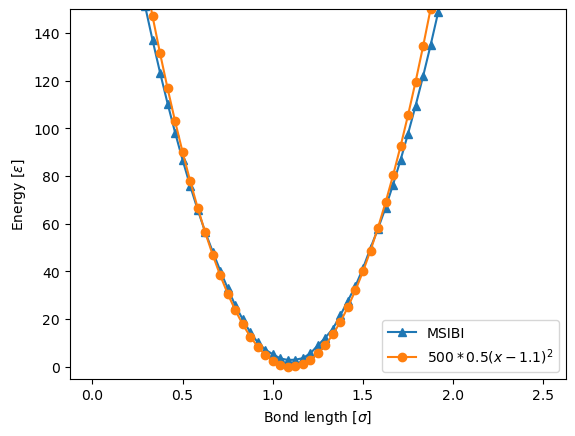
In most cases, the coarse-grained potential is not known ahead of time (hence the need for MSIBI, and other coarse-graining methods). However, for the purposes of this tutorial, we know that the target trajectory obtained from a simulation using a harmonic bond-stretching potential with the form of:
\(V(x) = \frac{1}{2}k(x - x_0)^2\)
where the parameters used were \(k=500\) and \(x_0 = 1.1 \sigma\). Below, we plot the final potential obtained from MSIBI against the known potential, and see that MSIBI was able to recover the bond-stretching potential purely from iterative adjustments in formed by comparisons between bond-length distributions.
[5]:
plt.plot(bond.x_range, bond.potential, label="MSIBI", marker="^")
plt.plot(
    bond.x_range,
    500 / 2 * (bond.x_range - 1.1) ** 2,
    label="$500 * 0.5(x-1.1)^2$",
    marker="o",
)
plt.ylim(-5, 150)
plt.legend()
plt.xlabel("Bond length [$\sigma$]")
plt.ylabel("Energy $[\epsilon]$")
[5]:
Text(0, 0.5, 'Energy $[\\epsilon]$')
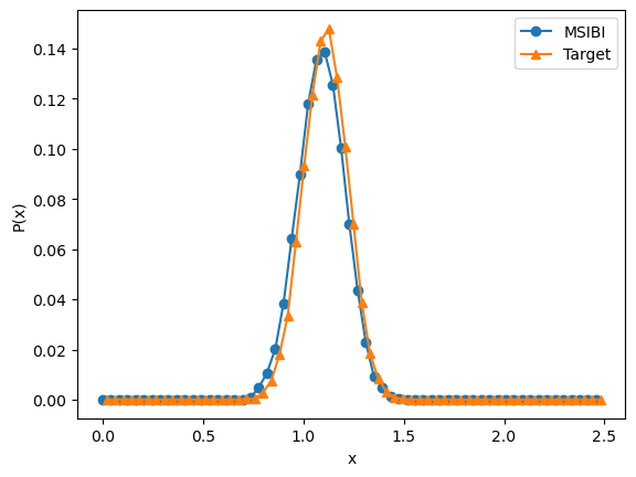
Here, we can compare the final bond-length distribution obtained from MSIBI against the target
[6]:
bond.plot_distribution_comparison(state=state)
2) Optimizing a bond-bending potential:
Many of the steps in this section are the same as in (1) optimizing bonds. However, there are a few differences.
We use the
set_harmonicmethod for theA-Abond. We could have saved the table potential from the last step and usedset_from_fileto create the A-A bond potential, but this illustrates another option for setting the potential for aForceobject. In this case, the potential obtained from MSIBI fits nicely to a supported bond-stretching potential in HOOMD-Blue, so we opt to use this instead. Note, thatoptimize=Falseis now used for theBondforce.An
msibi.Angleforce is introduced, and theset_polynomialmethod is used to create an initial guess potential.After optimization is finished, the table potential file is saved to a .csv file with
angle.save_potential("AAA_angle_potential.csv"). This will be used in the next step.
[7]:
# Remove the states directory created by the previous run
!rm -r states/

optimizer = MSIBI(
    nlist=hoomd.md.nlist.Cell,
    integrator_method=hoomd.md.methods.ConstantVolume,
    thermostat=hoomd.md.methods.thermostats.MTTK,
    thermostat_kwargs={"tau": 0.1},
    method_kwargs={},
    dt=0.0001,
    gsd_period=500,
    seed=50,
)

state = State(
    name="single-chain",
    kT=4.0,
    traj_file=os.path.join(str(target_data_dir), "single-chain.gsd"),
    n_frames=100,
    sampling_stride=2,
    alpha0=0.4,
)

bond = Bond(type1="A", type2="A", optimize=False)
bond.set_harmonic(k=500, r0=1.1)

angle = Angle(
    type1="A",
    type2="A",
    type3="A",
    optimize=True,
    nbins=60,
    smoothing_window=3,
    correction_fit_window=7,
    smoothing_order=1,
)
angle.set_polynomial(x_min=0.0, x_max=np.pi, x0=2.3, k2=80, k3=0, k4=0)

optimizer.add_state(state)
optimizer.add_force(bond)
optimizer.add_force(angle)
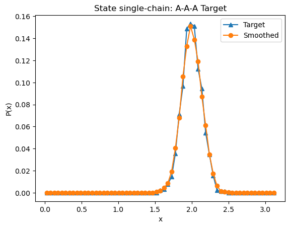
[8]:
angle.plot_target_distribution(state=state)
[9]:
optimizer.run_optimization(n_iterations=12, n_steps=5e5, backup_trajectories=False)
angle.smooth_potential()
---Optimization: 1 of 12---
Starting simulation 0 for state <class 'msibi.state.State'>; Name: single-chain; kT: 4.0; Alpha0: 0.4
Running on device <hoomd.device.CPU object at 0x15bc3e710>
Finished simulation 0 for state <class 'msibi.state.State'>; Name: single-chain; kT: 4.0; Alpha0: 0.4. TPS = 933386.1007608962

Force: A-A-A, State: single-chain, Iteration: 0, Fit score:0.380000

---Optimization: 2 of 12---
Starting simulation 1 for state <class 'msibi.state.State'>; Name: single-chain; kT: 4.0; Alpha0: 0.4
Running on device <hoomd.device.CPU object at 0x15bc3e710>
Finished simulation 1 for state <class 'msibi.state.State'>; Name: single-chain; kT: 4.0; Alpha0: 0.4. TPS = 939480.5424184859

Force: A-A-A, State: single-chain, Iteration: 1, Fit score:0.591111

---Optimization: 3 of 12---
Starting simulation 2 for state <class 'msibi.state.State'>; Name: single-chain; kT: 4.0; Alpha0: 0.4
Running on device <hoomd.device.CPU object at 0x15bc3e710>
Finished simulation 2 for state <class 'msibi.state.State'>; Name: single-chain; kT: 4.0; Alpha0: 0.4. TPS = 942134.1222136383

Force: A-A-A, State: single-chain, Iteration: 2, Fit score:0.708148

---Optimization: 4 of 12---
Starting simulation 3 for state <class 'msibi.state.State'>; Name: single-chain; kT: 4.0; Alpha0: 0.4
Running on device <hoomd.device.CPU object at 0x15bc3e710>
Finished simulation 3 for state <class 'msibi.state.State'>; Name: single-chain; kT: 4.0; Alpha0: 0.4. TPS = 944959.8675544249

Force: A-A-A, State: single-chain, Iteration: 3, Fit score:0.808889

---Optimization: 5 of 12---
Starting simulation 4 for state <class 'msibi.state.State'>; Name: single-chain; kT: 4.0; Alpha0: 0.4
Running on device <hoomd.device.CPU object at 0x15bc3e710>
Finished simulation 4 for state <class 'msibi.state.State'>; Name: single-chain; kT: 4.0; Alpha0: 0.4. TPS = 940898.4074353556

Force: A-A-A, State: single-chain, Iteration: 4, Fit score:0.884074

---Optimization: 6 of 12---
Starting simulation 5 for state <class 'msibi.state.State'>; Name: single-chain; kT: 4.0; Alpha0: 0.4
Running on device <hoomd.device.CPU object at 0x15bc3e710>
Finished simulation 5 for state <class 'msibi.state.State'>; Name: single-chain; kT: 4.0; Alpha0: 0.4. TPS = 939711.8467593096

Force: A-A-A, State: single-chain, Iteration: 5, Fit score:0.922593

---Optimization: 7 of 12---
Starting simulation 6 for state <class 'msibi.state.State'>; Name: single-chain; kT: 4.0; Alpha0: 0.4
Running on device <hoomd.device.CPU object at 0x15bc3e710>
Finished simulation 6 for state <class 'msibi.state.State'>; Name: single-chain; kT: 4.0; Alpha0: 0.4. TPS = 936562.8517964212

Force: A-A-A, State: single-chain, Iteration: 6, Fit score:0.951481

---Optimization: 8 of 12---
Starting simulation 7 for state <class 'msibi.state.State'>; Name: single-chain; kT: 4.0; Alpha0: 0.4
Running on device <hoomd.device.CPU object at 0x15bc3e710>
Finished simulation 7 for state <class 'msibi.state.State'>; Name: single-chain; kT: 4.0; Alpha0: 0.4. TPS = 945306.4589009112

Force: A-A-A, State: single-chain, Iteration: 7, Fit score:0.948889

---Optimization: 9 of 12---
Starting simulation 8 for state <class 'msibi.state.State'>; Name: single-chain; kT: 4.0; Alpha0: 0.4
Running on device <hoomd.device.CPU object at 0x15bc3e710>
Finished simulation 8 for state <class 'msibi.state.State'>; Name: single-chain; kT: 4.0; Alpha0: 0.4. TPS = 940714.3031846943

Force: A-A-A, State: single-chain, Iteration: 8, Fit score:0.936667

---Optimization: 10 of 12---
Starting simulation 9 for state <class 'msibi.state.State'>; Name: single-chain; kT: 4.0; Alpha0: 0.4
Running on device <hoomd.device.CPU object at 0x15bc3e710>
Finished simulation 9 for state <class 'msibi.state.State'>; Name: single-chain; kT: 4.0; Alpha0: 0.4. TPS = 933499.3717549229

Force: A-A-A, State: single-chain, Iteration: 9, Fit score:0.955926

---Optimization: 11 of 12---
Starting simulation 10 for state <class 'msibi.state.State'>; Name: single-chain; kT: 4.0; Alpha0: 0.4
Running on device <hoomd.device.CPU object at 0x15bc3e710>
Finished simulation 10 for state <class 'msibi.state.State'>; Name: single-chain; kT: 4.0; Alpha0: 0.4. TPS = 936754.1095402787

Force: A-A-A, State: single-chain, Iteration: 10, Fit score:0.968148

---Optimization: 12 of 12---
Starting simulation 11 for state <class 'msibi.state.State'>; Name: single-chain; kT: 4.0; Alpha0: 0.4
Running on device <hoomd.device.CPU object at 0x15bc3e710>
Finished simulation 11 for state <class 'msibi.state.State'>; Name: single-chain; kT: 4.0; Alpha0: 0.4. TPS = 936063.1430753793

Force: A-A-A, State: single-chain, Iteration: 11, Fit score:0.983333
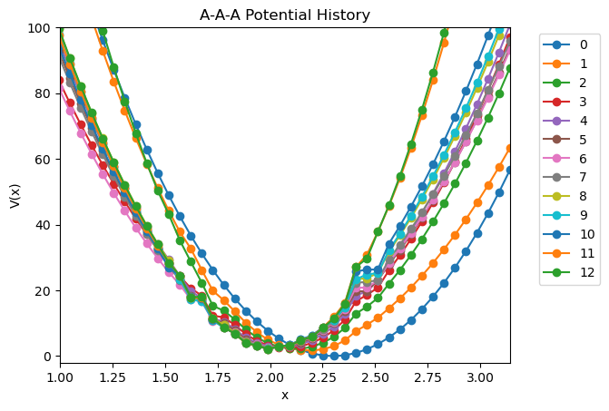
[10]:
angle.plot_potential_history(ylim=(-2, 100), xlim=(1, np.pi))
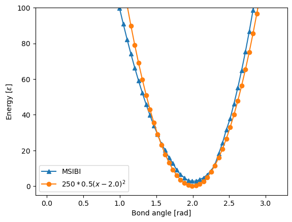
[11]:
plt.plot(angle.x_range, angle.potential, label="MSIBI", marker="^")
plt.plot(
    angle.x_range,
    250 / 2 * (angle.x_range - 2.0) ** 2,
    label="$250 * 0.5(x-2.0)^2$",
    marker="o",
)
plt.ylim(-5, 100)
plt.legend()
plt.xlabel("Bond angle [rad]")
plt.ylabel("Energy $[\epsilon]$")
[11]:
Text(0, 0.5, 'Energy $[\\epsilon]$')
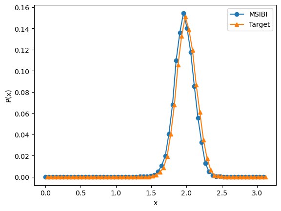
[12]:
angle.plot_distribution_comparison(state=state)
[13]:
angle.plot_fit_scores(state=state)
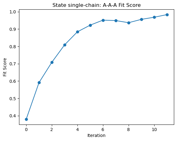
For this example, we will use the save_potential method to create a .csv file of the derived angle potential.
[14]:
angle.save_potential("AAA_angle_potential.csv")
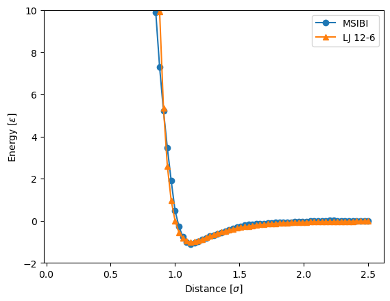
3) Optimizing a pair potential
Here, we learn the non-bonded pair potential from a target simulation of a “bulk” system containing 50 chains with 6 beads each. We follow the same procedure as the previous step to set the bond-stretching potential, use then use the set_from_file() method to set a bond angle table potential obtained in the previous step.
[15]:
# Remove the states directory created by the previous run
!rm -r states/

optimizer = MSIBI(
    nlist=hoomd.md.nlist.Cell,
    integrator_method=hoomd.md.methods.ConstantVolume,
    thermostat=hoomd.md.methods.thermostats.MTTK,
    thermostat_kwargs={"tau": 0.1},
    method_kwargs={},
    dt=0.0001,
    gsd_period=1000,
    seed=50,
    nlist_exclusions=["bond", "angle"],
)

kT = 3.0
state = State(
    name=f"{kT}kT",
    kT=kT,
    traj_file=os.path.join(str(target_data_dir), "3.0kT.gsd"),
    n_frames=200,
    sampling_stride=4,
    alpha0=0.7,
)

bond = Bond(type1="A", type2="A", optimize=False)
bond.set_harmonic(k=500, r0=1.1)
angle = Angle(type1="A", type2="A", type3="A", optimize=False)
angle.set_from_file(file_path="AAA_angle_potential.csv")

pair = Pair(
    type1="A",
    type2="A",
    optimize=True,
    r_cut=2.5,
    nbins=80,
    smoothing_window=11,
    smoothing_order=2,
    r_switch=1.5,
    correction_fit_window=7,
    exclude_bond_depth=3,
)
pair.set_lj(r_min=0.1, r_cut=2.5, epsilon=0.8, sigma=1.2)

optimizer.add_state(state)
optimizer.add_force(bond)
optimizer.add_force(angle)
optimizer.add_force(pair)
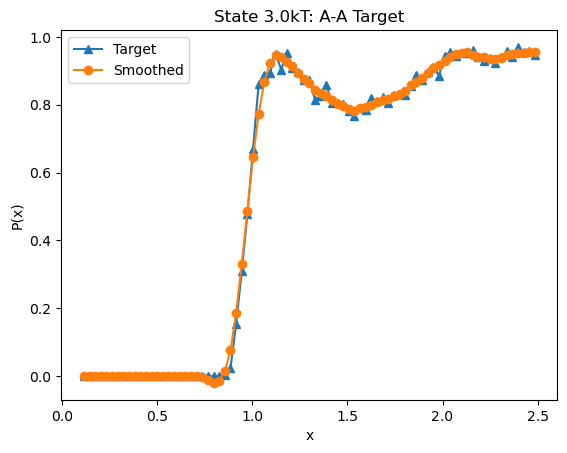
[16]:
pair.plot_target_distribution(state=state)
[17]:
for i in range(7):
    optimizer.run_optimization(n_iterations=1, n_steps=5e5, backup_trajectories=False)
    pair.smooth_potential()
---Optimization: 1 of 1---
Starting simulation 0 for state <class 'msibi.state.State'>; Name: 3.0kT; kT: 3.0; Alpha0: 0.7
Running on device <hoomd.device.CPU object at 0x15bc1f4d0>
Finished simulation 0 for state <class 'msibi.state.State'>; Name: 3.0kT; kT: 3.0; Alpha0: 0.7. TPS = 38036.9524428548

Force: A-A, State: 3.0kT, Iteration: 0, Fit score:0.917047

---Optimization: 1 of 1---
Starting simulation 1 for state <class 'msibi.state.State'>; Name: 3.0kT; kT: 3.0; Alpha0: 0.7
Running on device <hoomd.device.CPU object at 0x15bc1f4d0>
Finished simulation 1 for state <class 'msibi.state.State'>; Name: 3.0kT; kT: 3.0; Alpha0: 0.7. TPS = 37337.71070696939

Force: A-A, State: 3.0kT, Iteration: 1, Fit score:0.947908

---Optimization: 1 of 1---
Starting simulation 2 for state <class 'msibi.state.State'>; Name: 3.0kT; kT: 3.0; Alpha0: 0.7
Running on device <hoomd.device.CPU object at 0x15bc1f4d0>
Finished simulation 2 for state <class 'msibi.state.State'>; Name: 3.0kT; kT: 3.0; Alpha0: 0.7. TPS = 37016.4969941494

Force: A-A, State: 3.0kT, Iteration: 2, Fit score:0.969424

---Optimization: 1 of 1---
Starting simulation 3 for state <class 'msibi.state.State'>; Name: 3.0kT; kT: 3.0; Alpha0: 0.7
Running on device <hoomd.device.CPU object at 0x15bc1f4d0>
Finished simulation 3 for state <class 'msibi.state.State'>; Name: 3.0kT; kT: 3.0; Alpha0: 0.7. TPS = 36278.00181056251

Force: A-A, State: 3.0kT, Iteration: 3, Fit score:0.975935

---Optimization: 1 of 1---
Starting simulation 4 for state <class 'msibi.state.State'>; Name: 3.0kT; kT: 3.0; Alpha0: 0.7
Running on device <hoomd.device.CPU object at 0x15bc1f4d0>
Finished simulation 4 for state <class 'msibi.state.State'>; Name: 3.0kT; kT: 3.0; Alpha0: 0.7. TPS = 36894.53667176746

Force: A-A, State: 3.0kT, Iteration: 4, Fit score:0.986184

---Optimization: 1 of 1---
Starting simulation 5 for state <class 'msibi.state.State'>; Name: 3.0kT; kT: 3.0; Alpha0: 0.7
Running on device <hoomd.device.CPU object at 0x15bc1f4d0>
Finished simulation 5 for state <class 'msibi.state.State'>; Name: 3.0kT; kT: 3.0; Alpha0: 0.7. TPS = 36448.08990140063

Force: A-A, State: 3.0kT, Iteration: 5, Fit score:0.986809

---Optimization: 1 of 1---
Starting simulation 6 for state <class 'msibi.state.State'>; Name: 3.0kT; kT: 3.0; Alpha0: 0.7
Running on device <hoomd.device.CPU object at 0x15bc1f4d0>
Finished simulation 6 for state <class 'msibi.state.State'>; Name: 3.0kT; kT: 3.0; Alpha0: 0.7. TPS = 36459.91706098067

Force: A-A, State: 3.0kT, Iteration: 6, Fit score:0.991981
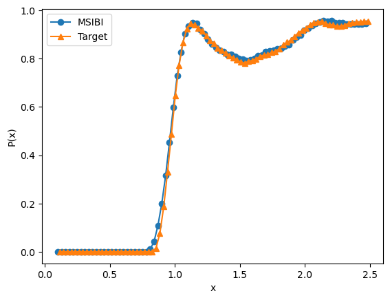
[18]:
pair.plot_distribution_comparison(state=state)
[19]:
from msibi.utils.potentials import lennard_jones
[20]:
plt.plot(pair.x_range, pair.potential, "o-", label="MSIBI")
plt.plot(
    pair.x_range,
    lennard_jones(r=pair.x_range, epsilon=1, sigma=1),
    "^-",
    label="LJ 12-6",
)
plt.ylim(-2, 10)
plt.legend()
plt.ylabel("Energy $[\epsilon]$")
plt.xlabel("Distance $[\sigma]$")
[20]:
Text(0.5, 0, 'Distance $[\\sigma]$')